How to Add Serial Numbers in Google Sheets: A Step-by-Step Guide

Adding serial numbers to your data in Google Sheets can help you organize and filter information much more effectively. Serial numbers give each entry a distinct identity, whether you’re keeping track of orders, managing inventory, or just making a list. Thankfully, there are easy ways to have Google Sheets produce consecutive numbers automatically. We’ll walk you through the steps of adding serial numbers to Google Sheets in this post.

Why Add Serial Numbers?

There are several uses for serial numbers in spreadsheet management:

Identification: They make it simpler to refer to certain entries by giving each row a unique identification.

Sorting and Filtering: You can efficiently sort and filter data using serial numbers, which makes it possible to put information in a meaningful order.

Data Integrity: You can keep your dataset error-free and free of duplicates by giving each entry a serial number.

Option 01: Using Fill Handle

The Fill Handle tool in Google Sheets allows you to automatically fill cells with a series of numbers, dates, or custom sequences. Easily create successive values by dragging the Fill Handle over a range of cells. This feature is particularly useful for adding serial numbers to your spreadsheet data.
Follow these simple steps to add serial numbers to your Google Sheets using the Fill Handle tool:

1. Enter the two Serial Numbers: Type the initial two serial numbers in the first two cells of the column you want to use. You might start with “1 & 2” or any other initial values, for instance.

2. Select the Cells: Click on both cells containing the initial serial numbers to select them.

3. Select Fill Handle and Drag Down: Move the cursor to the square/round(fill handle) at the bottom right corner of the selected cells a + icon will pop up. Click on the fill handle and drag down. Once you’ve reached the desired range, release the mouse button to apply the serial numbers.

Now you will have a series of numbers on the column

Option 2: Using SEQUENCE Function

The SEQUENCE function in Google Sheets generates an array of sequential numbers based on specified parameters. It simplifies the process of adding serial numbers by allowing you to define the starting value, the number of rows or columns, and the step size.

Select the Cell: Choose the cell where you want the serial numbers to start.
Enter the Formula: In the selected cell, enter the following formula:
=SEQUENCE(10, 1, 1, 1)

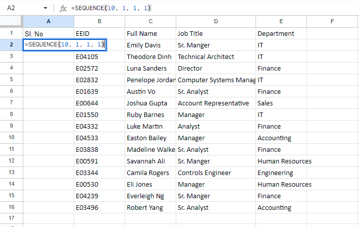
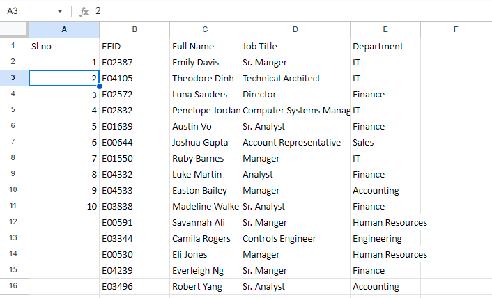
This formula generates a sequence of 10 numbers starting from 1 and continuing sequentially.

The number of rows in the sequence is specified by the first parameter (10). Adjust this value to the required length for the column containing your serial number. For instance, add 15 to fill 15 rows.

Start using the SEQUENCE function to add serial numbers in your Google Sheets today and experience improved data organization and efficiency!

Option 3: Using the ROW function

In Google Sheets, the ROW function outputs the cell’s row number. It is perfect for creating serial numbers in a spreadsheet because it can produce a series of consecutive numbers when used within an ARRAYFORMULA.

Follow these steps to add serial numbers to your Google Sheets using the ROW function:

Select the Cell: Select the cell where you want to start the serial number.
Enter the Formula: In the selected cell, enter the following formula:
=ARRAYFORMULA(ROW(A1:A10)-ROW(A1)+1)

This will create 10 serial numbers.

You can adjust the values to change how many serial numbers you need for example
=ARRAYFORMULA(ROW(A1:A15)-ROW(A1)+1)
This formula will generate 15 serial numbers from the cell you apply this formula to